Code
import numpy as np
import matplotlib.pyplot as plt
import os
import tensorflow as tf
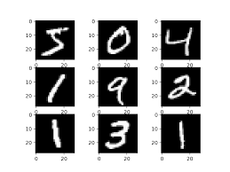
print("TensorFlow version:", tf.__version__)TensorFlow version: 2.14.0The MNIST database (Modified National Institute of Standards and Technology database[1]) is a large database of handwritten digits(0-9) that is commonly used for training various image processing systems.
import numpy as np
import matplotlib.pyplot as plt
import os
import tensorflow as tf
print("TensorFlow version:", tf.__version__)TensorFlow version: 2.14.0mnist = tf.keras.datasets.mnist
(x_train, y_train), (x_test, y_test) = mnist.load_data()x_train.shape(60000, 28, 28)x_test.shape(10000, 28, 28)y_train.shape(60000,)almost each number have ~6000 so total 60,000 on trainning
unique, counts = np.unique(y_train, return_counts=True)
dict(zip(unique, counts))
{0: 5923,
1: 6742,
2: 5958,
3: 6131,
4: 5842,
5: 5421,
6: 5918,
7: 6265,
8: 5851,
9: 5949}y_test.shape(10000,)the pixel values of the images range from 0 through 255. Scale these values to a range of 0 to 1 by dividing the values by 255.0
x_train, x_test = x_train / 255.0, x_test / 255.0model = tf.keras.models.Sequential([
tf.keras.layers.Flatten(input_shape=(28, 28)),
tf.keras.layers.Dense(128, activation='relu'),
tf.keras.layers.Dropout(0.2),
tf.keras.layers.Dense(10)
])loss_fn = tf.keras.losses.SparseCategoricalCrossentropy(from_logits=True)model.compile(optimizer='adam',
loss=loss_fn,
metrics=['accuracy'])# Show the model architecture
model.summary()Model: "sequential"
_________________________________________________________________
Layer (type) Output Shape Param #
=================================================================
flatten (Flatten) (None, 784) 0
dense (Dense) (None, 128) 100480
dropout (Dropout) (None, 128) 0
dense_1 (Dense) (None, 10) 1290
=================================================================
Total params: 101770 (397.54 KB)
Trainable params: 101770 (397.54 KB)
Non-trainable params: 0 (0.00 Byte)
_________________________________________________________________model.fit(x_train, y_train, epochs=3)Epoch 1/3
1/1875 [..............................] - ETA: 3:57 - loss: 2.2271 - accuracy: 0.1250 100/1875 [>.............................] - ETA: 0s - loss: 0.9847 - accuracy: 0.7128 202/1875 [==>...........................] - ETA: 0s - loss: 0.7288 - accuracy: 0.7853 306/1875 [===>..........................] - ETA: 0s - loss: 0.6125 - accuracy: 0.8190 412/1875 [=====>........................] - ETA: 0s - loss: 0.5378 - accuracy: 0.8422 514/1875 [=======>......................] - ETA: 0s - loss: 0.4939 - accuracy: 0.8560 617/1875 [========>.....................] - ETA: 0s - loss: 0.4638 - accuracy: 0.8656 721/1875 [==========>...................] - ETA: 0s - loss: 0.4325 - accuracy: 0.8742 825/1875 [============>.................] - ETA: 0s - loss: 0.4108 - accuracy: 0.8804 927/1875 [=============>................] - ETA: 0s - loss: 0.3913 - accuracy: 0.88581031/1875 [===============>..............] - ETA: 0s - loss: 0.3746 - accuracy: 0.89051134/1875 [=================>............] - ETA: 0s - loss: 0.3619 - accuracy: 0.89431238/1875 [==================>...........] - ETA: 0s - loss: 0.3484 - accuracy: 0.89821341/1875 [====================>.........] - ETA: 0s - loss: 0.3362 - accuracy: 0.90181444/1875 [======================>.......] - ETA: 0s - loss: 0.3262 - accuracy: 0.90461546/1875 [=======================>......] - ETA: 0s - loss: 0.3173 - accuracy: 0.90711645/1875 [=========================>....] - ETA: 0s - loss: 0.3107 - accuracy: 0.90921749/1875 [==========================>...] - ETA: 0s - loss: 0.3035 - accuracy: 0.91141850/1875 [============================>.] - ETA: 0s - loss: 0.2971 - accuracy: 0.91311875/1875 [==============================] - 1s 490us/step - loss: 0.2954 - accuracy: 0.9136
Epoch 2/3
1/1875 [..............................] - ETA: 1s - loss: 0.1279 - accuracy: 0.9375 107/1875 [>.............................] - ETA: 0s - loss: 0.1609 - accuracy: 0.9518 211/1875 [==>...........................] - ETA: 0s - loss: 0.1698 - accuracy: 0.9474 315/1875 [====>.........................] - ETA: 0s - loss: 0.1655 - accuracy: 0.9486 418/1875 [=====>........................] - ETA: 0s - loss: 0.1614 - accuracy: 0.9513 521/1875 [=======>......................] - ETA: 0s - loss: 0.1574 - accuracy: 0.9530 618/1875 [========>.....................] - ETA: 0s - loss: 0.1528 - accuracy: 0.9540 720/1875 [==========>...................] - ETA: 0s - loss: 0.1537 - accuracy: 0.9537 823/1875 [============>.................] - ETA: 0s - loss: 0.1516 - accuracy: 0.9545 926/1875 [=============>................] - ETA: 0s - loss: 0.1498 - accuracy: 0.95551028/1875 [===============>..............] - ETA: 0s - loss: 0.1481 - accuracy: 0.95631131/1875 [=================>............] - ETA: 0s - loss: 0.1467 - accuracy: 0.95671233/1875 [==================>...........] - ETA: 0s - loss: 0.1458 - accuracy: 0.95681336/1875 [====================>.........] - ETA: 0s - loss: 0.1445 - accuracy: 0.95761439/1875 [======================>.......] - ETA: 0s - loss: 0.1441 - accuracy: 0.95791541/1875 [=======================>......] - ETA: 0s - loss: 0.1439 - accuracy: 0.95791644/1875 [=========================>....] - ETA: 0s - loss: 0.1430 - accuracy: 0.95831747/1875 [==========================>...] - ETA: 0s - loss: 0.1425 - accuracy: 0.95841849/1875 [============================>.] - ETA: 0s - loss: 0.1421 - accuracy: 0.95841875/1875 [==============================] - 1s 489us/step - loss: 0.1419 - accuracy: 0.9585
Epoch 3/3
1/1875 [..............................] - ETA: 1s - loss: 0.0101 - accuracy: 1.0000 104/1875 [>.............................] - ETA: 0s - loss: 0.1184 - accuracy: 0.9642 206/1875 [==>...........................] - ETA: 0s - loss: 0.1109 - accuracy: 0.9657 307/1875 [===>..........................] - ETA: 0s - loss: 0.1103 - accuracy: 0.9646 411/1875 [=====>........................] - ETA: 0s - loss: 0.1105 - accuracy: 0.9647 513/1875 [=======>......................] - ETA: 0s - loss: 0.1120 - accuracy: 0.9649 616/1875 [========>.....................] - ETA: 0s - loss: 0.1133 - accuracy: 0.9652 718/1875 [==========>...................] - ETA: 0s - loss: 0.1118 - accuracy: 0.9654 820/1875 [============>.................] - ETA: 0s - loss: 0.1129 - accuracy: 0.9651 923/1875 [=============>................] - ETA: 0s - loss: 0.1124 - accuracy: 0.96511027/1875 [===============>..............] - ETA: 0s - loss: 0.1105 - accuracy: 0.96591130/1875 [=================>............] - ETA: 0s - loss: 0.1102 - accuracy: 0.96601235/1875 [==================>...........] - ETA: 0s - loss: 0.1092 - accuracy: 0.96601343/1875 [====================>.........] - ETA: 0s - loss: 0.1084 - accuracy: 0.96621446/1875 [======================>.......] - ETA: 0s - loss: 0.1095 - accuracy: 0.96621549/1875 [=======================>......] - ETA: 0s - loss: 0.1094 - accuracy: 0.96621652/1875 [=========================>....] - ETA: 0s - loss: 0.1085 - accuracy: 0.96641755/1875 [===========================>..] - ETA: 0s - loss: 0.1082 - accuracy: 0.96651859/1875 [============================>.] - ETA: 0s - loss: 0.1077 - accuracy: 0.96671875/1875 [==============================] - 1s 487us/step - loss: 0.1076 - accuracy: 0.9666<keras.src.callbacks.History at 0x2883a0e50>~accuracy: 0.9739 on testing data
model.evaluate(x_test, y_test, verbose=2)313/313 - 0s - loss: 0.0882 - accuracy: 0.9739 - 145ms/epoch - 464us/step[0.08815735578536987, 0.9739000201225281]predict_x=model.predict(x_test)
classes_x=np.argmax(predict_x,axis=1) 1/313 [..............................] - ETA: 8s172/313 [===============>..............] - ETA: 0s313/313 [==============================] - 0s 288us/stepperdition first 10
classes_x[:10]array([7, 2, 1, 0, 4, 1, 4, 9, 6, 9])real first 10
y_test[:10]array([7, 2, 1, 0, 4, 1, 4, 9, 5, 9], dtype=uint8)xxx.keras format not working at macos(2023-10-14) so using xxx.h5
model.save('my_model.h5',save_format='h5')new_model = tf.keras.models.load_model('my_model.h5')
# Show the model architecture
new_model.summary()Model: "sequential"
_________________________________________________________________
Layer (type) Output Shape Param #
=================================================================
flatten (Flatten) (None, 784) 0
dense (Dense) (None, 128) 100480
dropout (Dropout) (None, 128) 0
dense_1 (Dense) (None, 10) 1290
=================================================================
Total params: 101770 (397.54 KB)
Trainable params: 101770 (397.54 KB)
Non-trainable params: 0 (0.00 Byte)
_________________________________________________________________predict_x=new_model.predict(x_test)
classes_x=np.argmax(predict_x,axis=1) 1/313 [..............................] - ETA: 5s170/313 [===============>..............] - ETA: 0s313/313 [==============================] - 0s 291us/stepperdition first 10
classes_x[:10]array([7, 2, 1, 0, 4, 1, 4, 9, 6, 9])real first 10
y_test[:10]array([7, 2, 1, 0, 4, 1, 4, 9, 5, 9], dtype=uint8)https://www.tensorflow.org/tutorials/quickstart/beginner
https://en.wikipedia.org/wiki/MNIST_database